
The post goes from basic building block innovation to CNNs to one shot object detection module. Then moves on to innovation in instance segmentation and finally ends with weakly-semi-supervised way to scale up instance segmentation. The basic outline of the post is as described in the title and excerpt.
Feature Pyramid Networks
So, the journey starts with the now famous Feature Pyramid Networks [1] which was published in CVPR 2017. If you’ve been following the computer vision domain for the past 2 years, there are certain methods which are bound to be published, you just have to wait for someone to write it and train it and open source their code. Jokes aside, the FPN paper is truly great, I really enjoyed reading it. It’s not easy to establish a baseline model which everyone can build on in various tasks, sub-topics and application areas. A small gist before we go into detail - FPNs are an add-on to general purpose feature extraction networks like ResNet or DenseNet. Take any pretrained model of FPN from your favourite DL lib and voila use it like anything else!
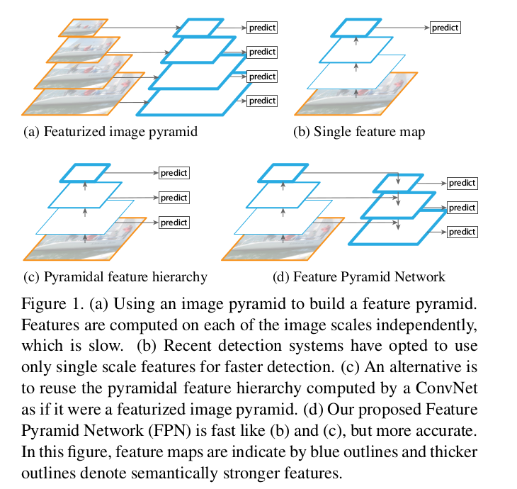
So, objects appear in various scales and sizes. Your dataset can’t capture all of it. So people use image pyramid (various downscales of the image) in order to make it easy for your CNN. But as you’d have guessed this is too slow. So people just use a single scale prediction, while some may take predictions from intermediate layers as well. This kinda is like the former one but its on the feature space. Easy way to imagine, put a Deconv after few ResNet blocks and get the segmentation output (similarly for classification, a 1x1 Conv and GlobalPool maybe). Lot of these architectures are now being used in another context of auxillary information and auxillary loss.
Moving to the topic, now, the authors found a clever way to improve on the above method. Instead of just having the lateral connections, put the top-down pathway as well to it. This makes perfect sense! Here, they use a simple MergeLayer(mode=’addition’) to combine both. A key point in this idea is, the lower level feature maps (initial conv layers let’s say) are not semantically strong, you can’t use it for classification. You trust the deeper level layers to understand that. Here, you also have the advantage of all the top-down pathway FMaps (feature maps) to understand it as good as the deepest layer. This is due to the combination of both lateral and top-down connections.
Some specifics
- A pyramid - all output maps which are of same size belongs to a stage. The output of last layer is the reference FMaps for the pyramid. Eg: ResNet - output of 2nd,3rd,4th,5th blocks. Depending on memory availability and specific use case, you can vary it however you want
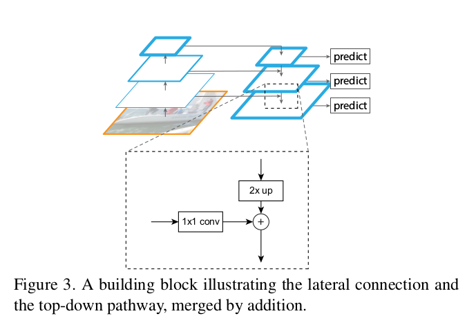
- Lateral connection: 1x1 Conv and Top-Down pathway is 2x Upsampling. The idea is from the top feature while going down coarse features gets generated (they use hallucinated I’m yet to fully read their actual paper which is named related to that) while the lateral connections adds the more finer details from the bottom-up pathway. I’ve borrowed a couple of figures from the paper which makes it super easy to visualize.
- Whats described in the paper is just a simple demo of sorts. Its to just show how well the idea works with simple design choices, so one shouldnt be afraid to dream a little bigger and more complex.
As I said earlier this is a base network which can be used anywhere, object detection, segmentation, pose estimation, face detection, all applied areas etc. Its only a few months old and already ~100 citations are there! The actual title is FPNs for Object Detection, so the authors go on to use the FPN as baseline in both the RPN (Region Proposal Network) and the Faster-RCNN networks. All key details are explained thoroughly in the paper but useful only to few people I guess so i’m just listing down some points from there.
Gist of experiments
- FPN for RPNs - Replace the single scale FMap with FPN. They have single scale anchor to each level (no need for multiscale as its FPN). They also show that all levels of the pyramid share similar semantic levels.
- FasterRCNN - They look at the pyramid in a way similar to output of image pyramid. So the RoI is assigned to a particular level using the formula.
- \(k\) = [\(k_0\) + \(log_2(\sqrt{wh}/244)\)]
- w,h is width, height. k is the level to which RoI is assigned. \(k_0\) is level to which w,h=224,224 should be mapped to.
- Gets SOTA on COCO without any bells and whistles as they call it (in all of the papers haha)
- They do ablation studies on each module’s working and thats how they’re able to prove the statements told in the beginning.
- They also show how it can be used for segmentation proposal generation as well based on the DeepMask and SharpMask papers.
- One should definetely read the paper (Section 5 onwards) if interested in the implementation details, experiment settings etc.
PS: One should note that FPN itself can be seen as a backbone on base ResNet and can be referred as such seperately too. A common way to refer has been Base-NumLayers-FPN eg: ResNet-101-FPN
Code
- [Official Caffe2]https://github.com/facebookresearch/Detectron/tree/master/configs/12_2017_baselines)
- Caffe
- PyTorch (just the network)
- MXNet
- Tensorflow
RetinaNet - Focal Loss for Dense Object Detection
It’s from the same team, same first author infact. This got published in ICCV 2017 [2]. There are two key parts in this paper - the generalized loss function called Focal Loss (FL) and the single stage object detector called RetinaNet. The combination of both performing exceedingly well in COCO object detection task, beating the above FPN benchmark also.
Focal Loss
This is pretty smart and simple! If your’re already familiar with weighted losses this is basically same with a smart weight to put more focus on classifying the hard and tough examples. The formula is given below, it should be self explanatory.
\[CrossEntropyLoss (p_t) = -log(p_t)\] \[FocalLoss(p_t) = -(1-p_t)^\gamma log(p_t)\] \[WeightedFocalLoss(p_t) = -\alpha_t(1-p_t)^\gamma log(p_t)\]\(\gamma\) is a hyper-parameter which can be changed. \(p_t\) is the probability of the sample from the classifier. Setting \(\gamma\) greater than 0 will reduce the weight for well classified samples. \(\alpha_t\) is the weight of the class as followed in normal weighted loss functions. In the paper its referred as \(\alpha\)-balanced loss. Note that this is the classification loss and is combined with the smooth L1 loss for the object detection task in RetinaNet.
RetinaNet
It was pretty surprising to see that a single stage detector was released from FAIR haha. Both YOLOv2 and SSD had been quite dominant in the single stage scene until now. But as rightly pointed out by the authors, they both havent been able to come very close to the SOTA methods. RetinaNet comfortably accomplishes that while being one stage and fast. They argue that the top results are due to the novel loss and not the simple network (where the backend is a FPN). The idea is that one stage detectors will face a lot of imbalance in the background vs positive classes (not imbalances among positive classes). They argue that weighted loss functions only target balancing while FL targets easy/hard examples and also show that both can be combined too.
Notes
- Two-stage detectors don’t have to worry about the imbalance due to the 1st step removing almost all of the imbalance.
- 2 parts - A backbone (A conv feature extractor eg: FPN) and two task-specific subnetworks (classifier and bbox regressor).
- Not much (performance) variations in the design choices of the components.
- Anchor or AnchorBoxes are the same Anchors from the RPN [5]. It is centered around a sliding window and associated with an aspect ratio. The size and aspect ratio are same as the ones used in [1] \(32^2\) to \(512^2\) and {1:2, 1:1, 2:1} respectively.
- At each stage of the FPN, we have the cls+bbox subnets which gives corresponding output for all locations in the anchors. This is shown in the Figure below
Code
Mask R-CNN
(Yaaay segmentation!) Mask R-CNN [3] is again by the same team (more or less). It’s published in ICCV 2017. It is for object instance segmentation. For the uninitiated, its basically object detection but instead of bounding boxes, the task is give the accurate segmentation map of the object! In retrospect one can say its such an easy idea, but making it work and becoming the SOTA and providing the fastest implementation with pretrained models is a tremendous job!
TL;DR : If you know Faster-RCNN, then its pretty simple, add another head (branch) for segmentation. So basically 3 branches, one each for classification, bounding box regression and segmentation.
Once again, the focus is on using simple and basic network design to show the efficiency of the method. They get the SOTA without any bells and whistles. (There are few complimentary techniques (eg: OHEM, multi-scale train/test etc) which can be used to improve accurac for all methods, bells and whistles implies not using them. As they’re complimentary, the accuracy is bound to increase. This isn’t in the scope of the paper is what they mean)
I really loved reading this paper, its pretty simple, yes. But lot of explanation is given for the seemingly simple things, in a clear way with experiments. For example, usage of multinomial masks vs individual masks (softmax vs sigmoid). Moreover, it doesn’t assume a huge amount of prior knowledge and explains everything (which can be a con sometimes too actually). One might find reasons as to why their obvious new idea (on an existing proven setup) didn’t work if one goes through this paper well. The following explanation assumes a basic understanding of Faster RCNN.
- It’s similar to FasterRCNN, two-stage, with RPN as 1st.
- Adds a parallel branch for predicting segmentation mask - this is an FCN.
- Loss is sum of \(L_{cls}, L_{box}, L_{mask}\)
- ROIAlign Layer instead of ROIPool. This basically doesn’t round off your (x/spatial_scale) fraction to an integer like in the case of ROIPool. Instead it does bilinear interpolation to find out the pixels at those floating values.
- For example: Imagine this, ROI height and width is 54,167 respectively. Spatial scale is basically Image size/FMap size (H/h), its also called stride in this context. Usually its 224/14 = 16 (H=224,h=14).
- ROIPool: 54/16, 167/16 = 3,10
- ROIAlign: 54/16, 167/16 = 3.375, 10.4375
- Now we can use bilinear interpolation to get upsample it.
- Similar logic goes into seperating the corresponding the regions into appropriate bins according to the ROIAlign output shape (eg 7x7).
- Checkout this python implementation of ROIPooling by Chainer folks and try to implement ROIAlign on your own if interested :)
- ROIAlign code is anyways available in different libs, check the code repos provided below.
- Backbone is ResNet-FPN
PS - I have written a seperate post as well on Mask-RCNN, it will be put up here soon.
Code
Learning to Segment Everything
As the title suggests, this about segmentation. More specifically, Instance Segmentation. The standard datasets of segmentation in computer vision are very small to be useful for real world. COCO dataset [7] which is most popular and rich dataset even in 2018 has only 80 object classes. This is not even close to being useful. In comparison, object recognition and detection datasets such as OpenImages [8] has almost 6000 for classification and 545 for detection. Having said this, there is another dataset from Stanford called Visual Genome dataset, with 3000 classes of objects! So, why aren’t people using this then? The number of objects in each category is too small, so the DNNs won’t really work on this dataset, so people don’t use this dataset even though its much richer and useful for real world! Note that the dataset doesn’t have any annotations for segmentation, 3000 classes of object detection (bounding boxes) labels only is available.
Coming to the paper [4], this is a pretty cool paper as well. As one can imagine, there’s not a huge difference between a bounding box and segmentation annotation in terms of domain, just that the latter is much precise than former. So since we have 3000 classes in Visual Genome [9] dataset, why not leverage that to give a segmentation output. That’s what they did, this can be called weakly-supervised (or weakly-semi-supervised as well?) learning, where you don’t have full supervision for the task you’re trying to achieve. It also can be associated with semi-supervised as they use both COCO+Visual Genome dataset. ie Both segmentation labels as well as bounding box labels. This paper is by far the most coolest 8-).
- It builds up on Mask-RCNN
- Trains on both inputs with mask and inputs with no mask.
- Adds a weight transfer function between mask and bbox mask.
- During training, one can backprop with bbox loss on the whole dataset but one can only backprop with mask loss for inputs which has mask groundtruth (dataset A)
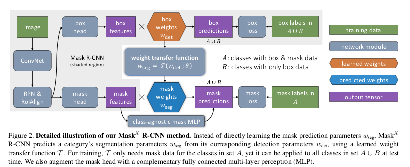
- During inference, when an input is passed, the function \(\tau\) predicts the weights to be multiplied with mask features. An extention (Section 3.4) of the model uses a fused MLP+FCN model to improve accuracy. Here, a simple MLP is used along with the above.
- This is shown in the figure below. A is COCO dataset and B is VG. Note the different losses for different inputs while (bbox and mask) outputs are calculated regardless.
- Backproping both losses will induce a discrepancy in the weights of \(w_{seg}\) as for common classes between COCO and VG there are two losses (bbox and mask) while for rest classes its only one (bbox). There’s a fix for this
- Fix: When back-propping the mask, compute the gradient of predicted mask weights (\(w_{seg}\)) wrt weight transfer function parameters \(\theta\) but not bounding box weight \(w_{det}^c\) .
- \(w^c_{seg} = \tau(\)stop_grad\((w^c_{det});\theta)\) where \(\tau\) predicts the mask weights.
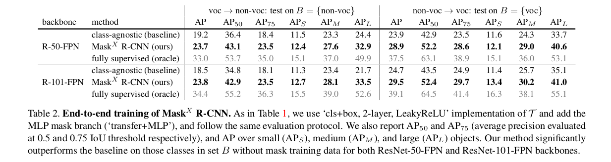
As they cant show accuracies on VG dataset since no annotations are available. So they take this idea to datasets on which results can be demonstrated. So PASCAL-VOC which has 20 classes and are all common in COCO. So, they train with segmentation labels from VOC and only bbox labels from COCO on those 20 classes. The results are shown on the task of instance segmentation on the 20 classes in COCO dataset. The same is done vice versa as well since both ground-truths are available in both dataset. This result is tabulated in below figure taken from the paper.
PS - I’m planning to write a blog on literature survey of papers which use weight prediction method to do impressive tasks, if it turns out to be useful.
Code
Acknowledgement
Thanks to Jakob Suchan for initial push to get more familiar with both Mask RCNN and Learning to Segment Everything papers!
References
[1] Lin, Tsung-Yi, Piotr Dollár, Ross B. Girshick, Kaiming He, Bharath Hariharan and Serge J. Belongie. “Feature Pyramid Networks for Object Detection.” *2017 IEEE Conference on Computer Vision and Pattern Recognition (CVPR)* (2017): 936-944.

[2] Lin, Tsung-Yi, Priya Goyal, Ross B. Girshick, Kaiming He and Piotr Dollár. “Focal Loss for Dense Object Detection.” *2017 IEEE International Conference on Computer Vision (ICCV)* (2017): 2999-3007.

[3] He, Kaiming, Georgia Gkioxari, Piotr Dollár and Ross B. Girshick. “Mask R-CNN.” *2017 IEEE International Conference on Computer Vision (ICCV)* (2017): 2980-2988.

[4] Hu, Ronghang, Piotr Dollár, Kaiming He, Trevor Darrell and Ross B. Girshick. “Learning to Segment Every Thing.” *CoRR*abs/1711.10370 (2017): n. pag.

[5] Ren, Shaoqing, Kaiming He, Ross B. Girshick and Jian Sun. “Faster R-CNN: Towards Real-Time Object Detection with Region Proposal Networks.” *IEEE Transactions on Pattern Analysis and Machine Intelligence* 39 (2015): 1137-1149.

[6] Chollet, François. “Xception: Deep Learning with Depthwise Separable Convolutions.” 2017 IEEE Conference on Computer Vision and Pattern Recognition (CVPR) (2017): 1800-1807.

[7] Lin, Tsung-Yi, Michael Maire, Serge J. Belongie, James Hays, Pietro Perona, Deva Ramanan, Piotr Dollár and C. Lawrence Zitnick. “Microsoft COCO: Common Objects in Context.” ECCV (2014).

[8] Krasin, Ivan and Duerig, Tom and Alldrin, Neil and Ferrari, Vittorio et al. OpenImages: A public dataset for large-scale multi-label and multi-class image classification. Dataset available from https://github.com/openimages

[9] Krishna, Ranjay, Congcong Li, Oliver Groth, Justin Johnson, Kenji Hata, Joshua Kravitz, Stephanie Chen, Yannis Kalantidis, David A. Shamma, Michael S. Bernstein and Li Fei-Fei. “Visual Genome: Connecting Language and Vision Using Crowdsourced Dense Image Annotations.” International Journal of Computer Vision 123 (2016): 32-73.